Correlation between two continuous measures

Sleep and activity

'...it's been a hard days night, and I been working like a dog.  It's been a hard days night, I should be sleeping like a log..'

We all generally assume that our activity and our sleep patterns are correlated, but what happens when we examine this relationship statistically?  Do we sleep more because we've been more active?  Or are we able to be more active because we've slept more? Or are we able to sleep more and be more active because we have more time to do both because of where they fall in our weekly cycle?  These questions can be examined directly, and in this section we'll explore the association using time series data collected from my Fitbit watch over a couple of months.  Please also check out all of the original code described in this discussion on Github.

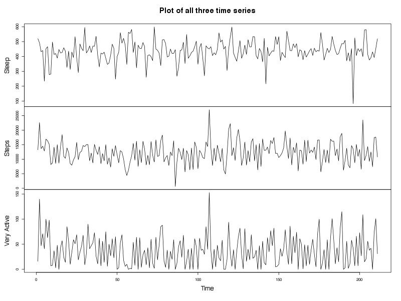
Time series for three continuous variables, collected by my Fitbit device.  Sleep (coded as 'Minutes.Asleep'), Steps, and Very Active (coded as 'Minutes.Very.Active').  The data has been filtered for days when less than 70% of a day was recorded.  

Fixed and Random

Let's start with a basic assumption, which we know is false but that we make all the time when we're creating regression models, which is that one of the variables is fixed (i.e., we can change it when we want, and measure it without error) and that one is random (the opposite).  If we make this assumption, then we can proceed using fairly standard regression approaches to see whether the value of one variable is associated with the value of another over time.  

Since we're most interested in sleep and activity, we'll fit five regression models: Sleep vs Very Active, Sleep vs Steps, Steps vs Sleep, Very Active vs Sleep, and Steps vs Very Active.  In each one, we'll examine the second variable as a regressor on the first.  To save time, we'll use the auto.arima function of the forecast package for R, and ignore seasonality for now.  We code the models in R like this:

auto.arima(Sleep, xreg = Steps)

Here's the results:
Model 1: Sleep~Very Active, ARIMA(0,0,0), Very Active coefficient -0.11, SE 0.16, t stat 0.67
Model 2: Sleep~Steps, ARIMA(0,0,0), Steps coefficient 0.00, SE 0.001, t stat 0.65
Model 3: Steps~Sleep, ARIMA(0,0,0), Sleep coefficient 2.36, SE 3.63, t stat 0.65
Model 4: Very Active~Sleep, ARIMA(2, 0, 2), Sleep coefficient -0.02, SE 0.03, t stat 0.6
Model 5: Steps~Very Active, ARIMA(1, 0, 0), Very Active coefficient 103.14, SE 4.61, t stat 22.36

Not very exciting.  It doesn't appear that we can say much about the relationship between sleep and either steps or exercise (Very Active).  Not unexpectedly, there's a clear association between Very Active and Steps, which perhaps could be interesting if we wanted to know if we took more steps on days in which we exercised, but overall not very informative.  Hopefully, we'll get more information when we start to look at lagged associations.

Lagged Relationships

We didn't see much when we looked at sleep and activity as occurring on the same day.  However, perhaps we'll have more luck when we start looking at the relationship across different time periods.  In this section we'll examine the cross-correlation coefficient between each of the variables, as well as look directly at the lagged relationship using regression models.  Since it's really hard to imagine a correlation going back past a week, we'll cut our CCF function at 7 days.  

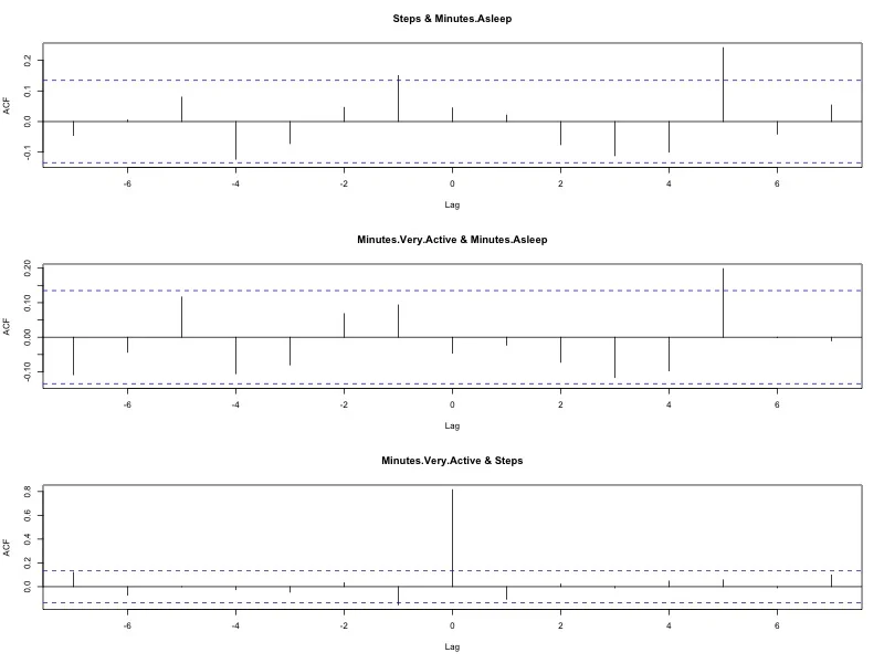
Cross-correlation functions between activity and sleep.  The lag at the bottom refers to the first variable listed--for example, in the first graph, the lag refers to the number of steps taken before or after the minutes of sleep was measured.

Again, nothing very exciting here with regard to sleep and activity.  There does appear to be a hint at a relationship between the number of steps taken the day before sleep, which we'll pursue below.  There's also something going on at 5 days out related to both steps and minutes asleep (5 days after activity, sleep is increased), but really hard to know what to make of that; common sense would suggest that it's more likely an outlier or reflective of another unmeasured confounder.  Let's start by looking at the lag-one day pattern using regression.  

First, it appears that the number of steps taken the day prior could be related to the hours of sleep.  This would seem to make obvious sense, but let's see what the numbers say:

Model 1: Sleep~Steps (Day - 1), R-square 0.022, p 0.029

It does appear that the steps taken the day prior are associated with more sleep that night.  Perhaps this is common sense, but it's nice to see it statistically.  Below we look graphically at the lagged relationships using a nice little function from the astsa package. 
 

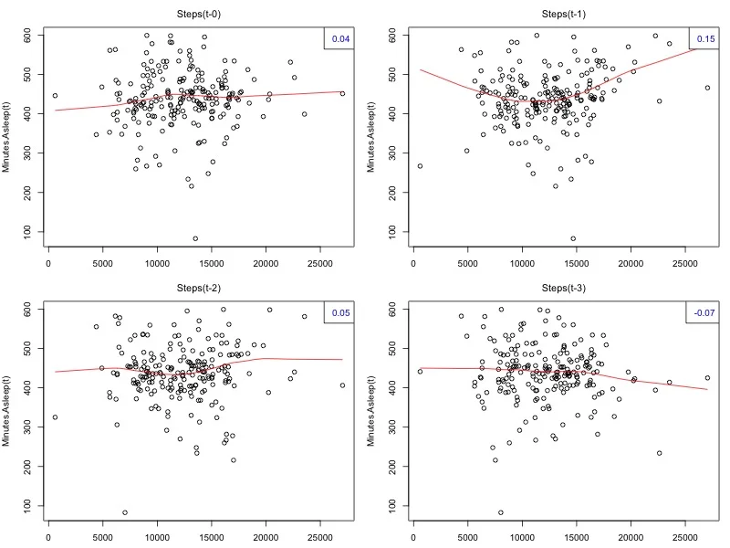
The lagged plot for Sleep based on lagged amounts of Steps.  Created using the lag2.plot function of the astsa package in R.  

Interestingly, when we look at the plot of this lagged relationship below, it appears that the relationship is actually nonlinear, with a U-shaped correlation between steps the day prior and sleep the following night.  This relationship suggests that up to about 11k steps, sleep is negatively correlated with steps the day before, but then after 11k, there's a positive correlation.  We can examine this effect statistically:

Model 2: Sleep~Lag.Steps+Lag.Steps^2,  R-square 0.044, p 0.0093

 It looks like the numbers also support that there is a nonlinear effect between steps taken the day prior and sleep, with a larger R-square value than the linear association above.  We can explore this relationship by fitting a line based on the amount of sleep predicted for each number of steps taken the day before.  

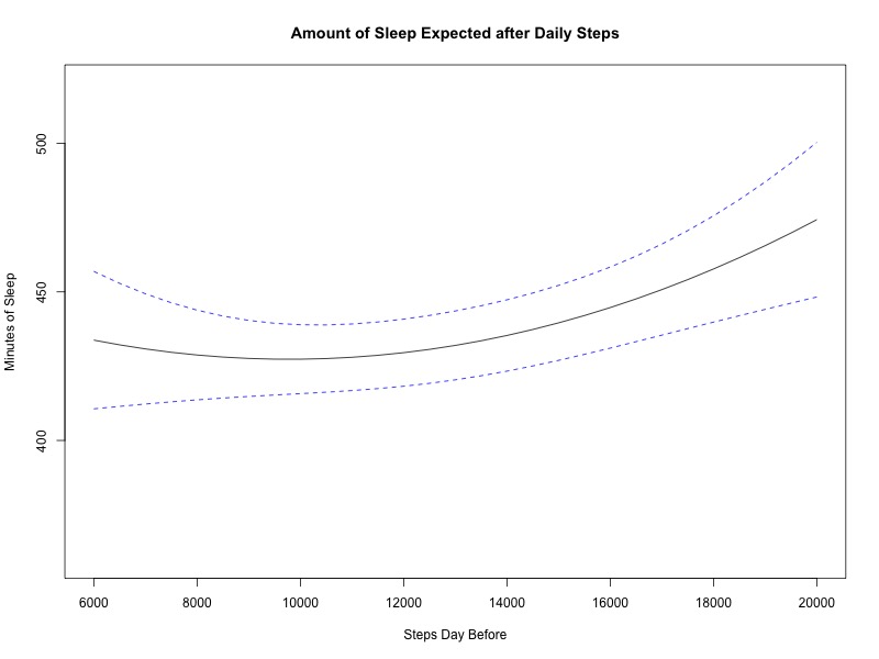
Predicted Minutes of Sleep after a given number of steps taken the day before based on our regression model.  Dashed lines are 95% confidence intervals.

Seasonality and Periodicity

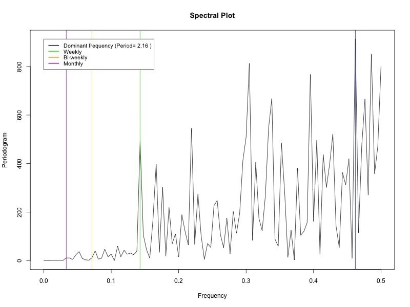
As a final look, let's make sure that our model is accounting for periodicity in the data.  As a focus on Sleep, we'll first examine the dominant frequencies of the sleep periodicity using a frequency domain method called the periodogram.  This graph, which was created using code from our Github page, displays lines for each of the main frequencies (daily, weekly, etc.), as well as the dominant frequency.  These curves are not smoothed, but as shown below, there is a pretty clear spike at a weekly period, which makes sense regarding sleep patterns.  For this reason, we will use a weekly (frequency = 7) period for final forecast models. 

As our final hurrah, we will now apply the weekly period to our ARIMA models to determine the impact of various numbers of steps taken the day prior on the minutes of sleep, after accounting for both seasonality and autocorrelation.  This 'forecast' graph allows us to predict various lines for the minutes of sleep we would expect to obtain depending on the number of steps taken the day prior.  As shown below, one could expect to get about 50 extra minutes of sleep the following night depending on how many steps were taken. 

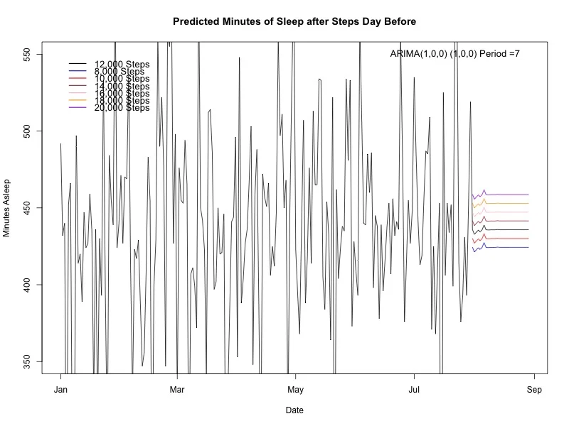
Based on auto.arima, which selected a seasonal model with AR1 and SAR1 components around a period of 7.  The astute person might note that the U-shaped quadratic relationship was not captured here, which is primarily due to a limit in the auto.arima function, which only allows a single xreg variable, rather than both the linear and quadratic predictors.  

So, we've successfully demonstrated that the Beatles were correct.  If I've been working like a dog, then statistically speaking, I should be sleeping like a log (at least if I'm not on the lower limb of the quadratic prediction line).  So where does this leave us?  

Like any analysis, we need to consider the following key criteria:

1. Have we demonstrated a significant correlation?
2. Are we powered to state that there is no correlation?
3. What are the assumptions and potential biases in our analytical approach?

We also need to consider a couple other issues.  For one, how might we truly automate this analytical process?  Clearly, the quadratic relationship was only picked up from manual review of the lagged correlation plots.  We could potentially include a quadratic term in all analyses and examine for significance, but this would create a large number of extra analyses, most unnecessary.  Two, should we include 'common sense' in our evaluation?  We didn't pursue the lag-5 relationship with sleep and activity because it didn't make much sense how one could effect the other 5 days later.  This would seem to reflect more of a seasonal pattern, but perhaps there's also something we're missing.  Is it possible that a good night's sleep on Monday will be reflected in a more active Friday?  Finally, this dataset is part of a dynamic process for collecting data, which can change over time, all the more so if I perform an analysis and decide that I should try to get more steps the day before if I want to sleep more.  How do we manage this dynamic situation?  Are there Bayesian or other methods that can use the data already collected to build more or less confidence around a given correlation?  If we plan to apply these methods to hundreds or thousands of people wearing activity monitors, we're going to need to solve these and other problems...

As always, please leave any comments or suggestions below.